note: currently working on a remake of SpaceCore, I’ll update this page to reflect that at some point. until then, it’s gonna remain half-assed and nonsensical
Ok I’ve had too many stupid arguments with too many people, so I’m just gonna put this here aight
Why am I writing the entire game & engine from scratch, instead of using one of the myriads that exist already?

- Those “myriads of engines” are almost exclusively made for walking around in 3d-first-person-perspective on a pre-made flat arena and shooting people (or “general purpose” 2d/text engines, which (for me) are easier to remake from scratch than to actually use (see exhibotanist for an example), or very specific engines made for very specific games, which are more “interesting examples” to look at and mess around with than something you actually use to make something else out of). The game I want to make does none of that
- Unlike all the youtubers and (most) blogposters out there, I am more interested in making something that’s actually worth it, rather than shooting out something as quickly as possible that catches the most attention and gets me a lot of money, but is, in the end, pretty pointless
- Partially repeating the last point, but I am more interested in implementing interesting and convoluted mechanics than I am in finishing this as a game and bringing it out. Which also means I’m going to implement a LOT of stuff that is either going to be very irrelevant for the final gameplay (eg elaborate computer control systems), or just straight-up does not make it into the project (eg multiple elaborate inventory systems, voxel-based renderer, NPC AIs with synthesized voices).
So, with that out of the way,
   ____                  _____
  / __/__  ___  _______ / ___/__  _______
 _\ \/ _ \/ _ `/ __/ -_) /__/ _ \/ __/ -_)
/___/ .__/\_,_/\__/\__/\___/\___/_/  \__/
   /_/
SpaceCore was born in ‘19 after a couple thousand hours in KSP and quite a bit of disappointment with my space station. I read up on orbital mechanics, found out they were incompatible with the way KSP handles physics, and after looking through multiple game engine options, I settled for writing one myself from scratch.
It is planned to be part ship builder and flyer (ala KSP), part planet/asteroid miner (ala minecraft/space engineers), part MMORPG (ala WoW).
Elite (‘84) was the main inspiration for the aesthetics. It is not intended to be “aesthetically advanced” - I am a big fan of retro graphics and code that doesn’t do unnecessarily more than what it should, and I strongly believe that the game industry’s obsession with photorealism has been detrimental.
Working so far:
- Raster graphics
- Octtree-based n-body orbital mechanics - including gravity torque
- Cube-marched LOD terrain
- Ship softbody simulation
Not working so far:
- Collisions
- Inventory system - or anything player related for that matter
- Ship builder
- Planet materials & athmospheres
- All player-related stuff (besides basic camera settings)
- All internet-related stuff
Contents
- Specifics
- Interpolation
- Orbital dynamics
- Octtrees
- Gravitational torque
- Softbodies
- Bullet rigid-body physics
- GJK-EPA rigid-body physics
- Rasterisers
- LoD
- Raytracers
- Perlin noise
- Marching Cubes
- Dynamic LoD
- Parsers
- Screenshots
Specifics
Now, what exactly does it do? First, let’s look at how the main inspiration does what it does. KSP uses something called “patched conic approximations” to simulate orbital dynamics, the Bullet physics engine) (or some variant thereof) for collisions, and mumble mumble LOD for terrain graphics (afaik Bullet implements its own LOD collision meshes?). Worst of all, it’s made in Unity. Let me tell you about Unity. Unity is terrible - and no I’m not talking about the shitty pricing practices, those are terrible but not even the worst issue. Have you ever been exasperated that the game takes ~20min to start every time, longer with mods? Unity needs that time to convert all the game assets from its proprietary memory format to its proprietary runtime format. Ever been pissed that even with all settings set to their lowest value, the game still runs like a rusty three-wheeled trabant low on gas? Unity only permits one physics thread, with very minimal optimisation. The insane difficulty of developing any memory introspection (fortunately greatly alleviated by preexisting mods)? Unity. It’s like java - a buncha hacks that haven’t had to program aything decent in their lives decided it was good because it had sufficient bloat, and unfortunately those hacks had screwed over enough people to get a teaching position - and because all the tutorials and courses are for unity, that’s what people learned, regardless of how terrible those tutorials and courses are.
Tldr if you want to make a game, either use Godot or something similarly open, or learn how to make it from scratch.
Interpolation
Interpolation is the trick of taking two points and picking another point that lies “between them”. It’s not a big part of SpaceCore like the rest, but it is a neat trick that gets used over and over, so I decided to give it a dedicated section.
XXX
Orbital dynamics
KSP’s orbital mechanics use something called “patched conics”. As our buddy Kepler pointed out a while ago, if you only have two bodies orbiting each other, you only need conics (circles, ellipses, parabolas, hyperbolas) to describe their orbits. “Patched conics” takes that idea and runs with it, reducing any system to pairwise attraction between objects (via “spheres of influence”) to determine which body gets which satellites, and “patching” between those). This is neat, because it allows you to time-warp arbitrarily (as long as you can keep up with the patches), but it does away with a lot of cool shit like tidal locking (1) or lagrangians. The “better” method are n-body differentials - since every object in the universe attracts every other object in the universe, we can just go through each pair of objects, and use the good old formula of gravitational attraction to figure out the forces. If we then also treat every object (eg ship) as a collection of smaller parts (bound together as a softbody for example) (in common english, “a buncha stuff connected with duct tape and rubber bands”), we can also simulate torque (see below). As you can imagine, however, performing anything “for every pair of objects in the universe” is kind of very computationally expensive (in common english, “slow”), so we use another neat little programmer trick called “octtrees”. Short explanation of that is that instead of performing something “for every object within this region of space”, we can first construct a fancy structure representing the different regions, and then perform the thing on space itself. Sounds fake - we need to generate a weird region structure every cycle? - but it lets us do some neat optimisations that turn out to put it in a significantly better computation class (from O(n2) to O(n log n)) (aka “a damn lot faster”).
1: SPC originally came to be because I was annoyed that my space station didn’t keep rotating when I time-warped - an effect known to most players and often used to stabilise aircraft when the kraken pays a visit, but very much not cool when you want a fancy setup.
Octtrees XXX
Gravitational torque
Very short explanation of gravitational torque: if an object (A) passes by a heavier object (B), the parts of A closer to B are pulled at stronger than the parts further away - thus, A begins to spin. This doesn’t usually happen in simulations because of how we simulate objects - as far as (orbital) physics is concerned, we treat all objects as points with masses. This works out well enough to simulate the relative positions of bodies (since all points have is a position), but ignores effects like aforementioned tidal locking.
While it would be theoretically possible to simulate masses as actual volumes with density, that ends up being very impractical (after all, it’s one step separated from treating objects as collections of atoms and running quantum physics on them - which doesn’t pan out well beyond about a dozen atoms). Instead, we take the metaphor a step further - each ship is now a collection of parts (and those parts are points with masses). Now, we can calculate gravitational forces for each part of the ship. The average of those (sum up, divide by number of parts) is the force acting on the ship, and the deviance from that (subtract average from forces on each part) are the parts acting only within the ship - which we can use to simulate tidal forces.
For practical reasons, we only simulate the current ship as a collection of parts - in other words, we don’t simulate forces between every single pair of bolts, but go through all ships and only simulate that ship individually, using the octtree from above to approximate the effects of all other ships. It is still an order of magnitude slower (if the average ship has N parts, it takes about N times longer to simulate orbital dynamics), but fortunately it is still within the same complexity class, meaning we don’t really need to bother doing programmer black magic to optimise it further.
Softbodies
Above, I described softbodies as “a buncha stuff connected with duct tape and rubber bands”. That ends up being a surprisingly accurate and useful description. We model each ship as a bunch of parts with a location and a mass - the softbody simulation deals with how those partss are connected. Specifically, it keeps a list of connections between them. Those connections have a list of relevant properties - length, twist, elasticity - of which we pick which ones are relevant. Each time step, the simulation calculates how far the current partss are deviating from those constraints, and nudges them in the opposite direction - much like a stretched rubber band will try to pull its ends back together.
Implementation-wise, this is about as straight-forward as it gets. The main difficulty is in figuring out the math for the constraints (distance between two points is easy - it’s just middle-school pythagorean. the twist between them gets a lot more complicated), and then running those equations backwards (multiplied by some damping factor - which you can also make arbitrarily complicated to suppress KSP-style wobbling) to “nudge” them back. Some engines use huge matrices to figure out all relevant constraints at once, but the calculation and application of those matrices is usually much slower than just iterating through the constraints (also very inflexible to adding more or more complicated constraints), and while they may brag their ability to satisfy all constraints at once, this usually turns out to not be relevant - as all the constraints are in a single continuous system (“keep running against each other”), they end up taking care of each other (the beauty of differentials, amirite?)
Bullet physics engine
The Bullet physics engine) is a physics engine widely known for providing a “precise” and “easy to use” solution for a lot of physics-related stuff like collisions, softbodies, fluids (I think? Pretty sure they at least considered it), dynamics (“moving platforms pushing stuff around”), and much more. The quotation marks are because I went digging through the code for parts I could use (instead of just including it as a library and using the wrappers like an econ student down on his last three yachts) - and boy lemme tell you, that code was almost entirely wrappers, and what wasn’t wrappers was left unmodified from the original doctoral thesis that presented the algorithm. So I scrapped that and went to implementing that instead. Come to think of it, this section was pretty useless, let me redo it.
Bullet GJK-EPA physics engine
The “Gilbert-Johnson-Keerthi expanding polytype collision algorithm” is an algorithm (“buncha code”) that takes two convex shapes and returns whether they are intersecting (“bumping”), and if so, the intersection depth (“how bent your bumpers are afterwards”). If you think the name sounds intimidating, you ain’t seen shit - this part alone took me over a year, and I still haven’t managed to get it working properly. There’s a reason the physics engine is the one piece of code you absolutely do not write yourself. I’ve had actual nightmares from it.
How it works (trigger warning for math, proceed at your own risk): a rigid object (“stuff you can bump against”) is, mathematically speaking, a set of points in space (specifically, the points we consider “inside” the object). If two objects are intersecting, then there are points that appear in both sets. Thus, if we subtract all points from one set from all points of the other, the resulting set (called the Minkowski difference of the two) contains the origin iff the original sets overlap. If we then also add the restriction that the sets have to be convex (meaning, any two points within a set form a line that must also be entirely contained in the set) (“no dents”), we can limit the search to surface points, requiring the origin to be enveloped - which is a lot faster, because instead of searching for a pair of points on both objects that are equal (which would require us to search all possible pairs if there isn’t a match), we only need to find four pairs that construct a shape that envelops the origin (which we can abort early on if we find a separating axis to the origin). This is also neat, as the models required are (almost, because convex) identical to the models we already use for graphics.
In practice, GJK starts with a random point (in our case, the one furthest along the X axis) and keeps picking points that are further towards the origin from it (a point “furthest in some direction” is known as a support - and we know those to be enough because of the convex restriction from above) to construct a simplex (line, triangle, tetrahedron aka d4 aka “the pointy die that hurts to step on”), and then checks if that simplex contains the origin (which is easy, because checking where a point is in relation to those shapes is pretty easy, mathematically speaking).
XXX include math for that?
If we manage to contain the origin, we have a collision. The issue then is that the shape that GJK terminates at (a simplex subset of surface points from the minkowski difference) is (usually) one made from points that are “as far away as possible” from the origin, when we’d ideally like to have close ones (so we know where the collision actually takes place). That’s the second part of the algorithm: EPA takes the resulting tetrahedron as its original polytype (“fancy shape”), then repeatedly looks for the point in it (well, point on a face) closest to the origin, and replaces it by the minkowski difference support in its direction (I like to think of it as “poking the triangle”, which sounds like something from a porn parody of Flatland). If we pick the same point twice, that means it’s the closest point in the minkowski difference as well - in other words, the closest points on the two objects.
XXX example, also the poking is more complicated than it sounds
Raster graphics
Are you not glad you opened this page and read all that math above? Are you not glad you thought to yourself “SpaceCore, huh? Custom game engine? I wonder how that works!”? Are you not happy with your life choices that led to you reading that? I hope you are. Now how about we do something easy as a treat.
Rasterisers are the most common way of doing computer graphics. Vast majority of graphics you’ve seen, it was raster graphics. You know the “it’s all triangles” memes? Yeah that’s raster graphics: each object is a list of triangles, and each triangle is a list of three points in 3d space (plus maybe three points in 2d space, telling us how to map a texture to it) (fun fact: you can also use 3d points for textures as well, and then you can do real funky shit with volumetric textures). Since pretty much all 3d points (known as “vertices”) will be shared between triangles, you usually keep a list of all points in an object, and then have the triangles index that instead (that way, you only do math once per point, instead of once for each triangle that point appears in). Since we have to draw so many triangles, it is important to make sure that drawing each of them is as fast as possible - that’s the reason GPUs are so popular. I won’t explain GPU rendering however, as SPC explicitly only uses a software renderer (meaning, all graphics are done on the same chip and in the same process environment as all other calculations) - the math is the same though, and GPU rendering only differs in compilation and memory management - both nasty side-effects of modern programming that we will not be covering.
To actually render the object on screen, we need two steps - figuring out where each triangle goes on the screen, and then actually drawing the triangles. For the first step, we need to figure out where the triangles are in relation to the camera - a common explanation for this is that we keep the camera fixed so we can do math to it, and rotate the world around it. The rotation (and translation) is usually done by rotation (and translation) matrices (you take the location and rotation of the camera and use them to create a matrix (“weird math object”) that is a bit like a function for lists") which when applied to vertices transforms them from global to camera-local space). Sound complicated? Agreed - I just used quaternions. Quaternions are like vertices, but in 4d space - which just means I store four values for each of them instead of three. The neat thing about them is that the additional dimension lets them act as vertices AS WELL AS the matrices applied to them, and they don’t suffer from a lot of the mathematical issues rotation-translation matrices suffer from, like gimbal lock or explicit trigonometrics (thanks Hamilton!) (no not that one, the other one). They are also a little bit faster - assuming you remember to renormalise them properly. Pretty much the only downside is that quaternion multiplication - the thing that makes this all possible - is a bit complicated, but you can just copy the matrix for that from wikipedia and call it a day. Thus, a camera is two quaternions, one for location and one for rotation, and we can just multiply and add those to each vertex to figure out where it goes on the screen. Easy!
XXX example matrices and quaternions
The second part is taking the three points on the screen and actually figuring out which pixels to fill in to make it look like a triangle. This turns out to be a bit more complicated. Let’s say we have the three points A, B, and C on the screen. Since it doesn’t matter which order they are in, let’s say A is the uppermost one (lowest X coordinate) and C the lowermost one (highest X coordinate), with B between them. Then, our triangle would look something like this (with helpful coordinate hints):
 y->
x  A
| / \
v.   \
 /    \
 B     \
  `-_   \
     `-_ \
        `-C
While we’re at this, let’s add another point D that is on the AC line at the height of B:
   A
  / \
 .   \
 /    \
 B-----D
  `-_   \
     `-_ \
        `-C
If it so happened that B was further to the right than C in the beginning, we can swap B and D here to fix that. Now we’ve separated our triangle into two other triangles (I promise this is an improvement). There are B.x-A.x lines of pixels in the upper triangle. Each line L is thus L/(B.x-A.x) of the way between A and B, its Y coordinate is thus also that far between the Y coordinates of A and B - or in terms of code, L*(B.y-A.y)/(B.x-A.x) (this is called interpolating and is very useful if you need to find something that is so-and-so-far between other somethings) (we can get rid of the division (division is slow on computers) by using something called Bresenham’s line algorithm, but that’s a bit complicated for right now). For texture mapping, we can interpolate the texture coordinates of the points in the same way we interpolate their position on the screen, and use the result to pick a color from the texture. The reason we separated our triangle in two triangles is that by using C instead of A (and flipping some of the signs), we can draw the bottom triangle in the same way!
There is actually one more little trick we’ll need for triangles. We have to know which triangles are in front of each other. We can do this with the painter’s algorithm (significantly easier to implement), or with a depth buffer (needs a bit more memory and some more math, but is significantly better in pretty much every aspect). When we calculate the screen location of each point, we also get their depth. The painter’s algorithm works by first sorting all faces by their depth, and drawing the farthest ones first - that way, all faces that are closer get drawn on top. Unfortunately this requires sorting all the faces, which can get very slow, and it also doesn’t account for special cases like faces intersecting. A depth buffer requires us to store the depth at each pixel. Using much the same code we used for figuring out the points for the triangles, we can figure out the depths of those points, and if they are closer than the current point at that pixel, we draw over it.
LoD
Levels of Detail are a neat little trick rendering engines use to make their lives easier. If you are next to a spaceship, you can see every dent and scratch on her hull. If she’s on the other side of the solar system however, you’d be lucky if she showed up even as a single pixel on your screen (well, I like the non-anti-aliasing aesthetic and didn’t implement pixel smoothing, so she will). In that case, why bother rendering all the dents and scratches on that single pixel? For that matter, why bother rendering all her parts to begin with? That’s where LoDs come in - each model has multiple versions, each with less detail than the previous. Thus, for a distance from the object, we can pick a model that shows enough to look right, but little more so we can save up on time and resources. This is easily done via a quick distance check and then picking an appropriate model from a list when rendering - since it’s an easy calculation done once per model (compared to the millions of calculations we need to do for eg pixelating the triangles) and has a huge effect on rendering (could turn all those millions of calculations into a single pixel), it is not something we need to optimise.
Raytracers
SPC does not use a raytracer, however I did toy with the idea (and wrote a couple different raytracer implementations to see how it’d work). As raytracers are also commonly known as “the other rendering technique”, I thought they’d be interesting enough to go over as well.
While rasterisers are made from the same math approximations that computers work with, raytracers take a more physical approach. What is this “seeing” thing about really? A bunch of light falling onto an image sensor. What is “light” really? A bunch of light rays (1) being emitted, bouncing off some objects, and then ending on the image sensor. What does “bouncing off some objects” mean? That largely depends on the objects. Raytracers model objects as mathematical equations, giving us an easy way of figuring out the “normals” (“which way is this bit facing?”) and thus optic properties of objects (which depend locally on the normals (eg which way reflections are cast), and globally on properties we can set manually (“which color is this object?”)). This lets us use the same models as with rasterisers (by using a formula defining a triangle as a plane between three points) (this is significantly slower than rasterisers, because we have to actually search for a triangle colliding with a ray - although there are also algorithms improving on this), but it also lets us use and render mathematical objects that would otherwise be very difficult or impossible to work with, like Nurbs spheres or Mandelbulbs.
A neat usecase is that raytracers work really well when combined with octtrees. Raytracers require us to be really good at figuring out what objects rays collide with. This is usually very slow (because you have to check every object) or very complicated (space partitioning algorithms), but we can use the recursive, axis-aligned nature of octtrees to speed it up significantly at almost no cost. Recursively iterate through nodes, with each node needing six checks (two per axis - one for the nearest surface, and one for the middle one) that can be hardcoded and optimised a lot. Coding visualisers, for example for ship parts or voxel-based (“minecraft-like”) worlds, thus becomes easy - and fun!
XXX examples
1: The clever walnuts among you might be thinking “A-ha, you nerd, but light is not just a wave, it’s also a particle!” If that is you, give yourself a pat on the back from me. For purposes of raytracing, we treat light as rays, because that is how optics work. Some raytracers do not treat rays as being straight lines, but as geodesics - which lets you model cool shit like gravitational warping or non-euclidean spaces. Another one actually takes Heisenberg’s uncertainty principle into consideration, and treats light as quanta. This is what raytracing excels at - modeling weird stuff light does.
Perlin noise
We need to actually generate “realistic-looking” (or at least, interesting) terrain for the planets/asteroids. The standard approach for this, used in almost every single computer game since Rogue, is “make some Perlin noise and slap some filters on that”. It would be trivial to get a library to do that for me, but I have the ethos to code every piece of SpaceCore myself - fortunately, writing a noise library is rather easy.
Perlin noise was introduced in XXX for generating “realistic-looking” noise for computer graphics. There are other ways of generating (mathematical) noise that are more “realistic” (XXX), but Perlin noise has the benefit of being almost dead-simple to make.
Let’s see an example in action. First, pick some random numbers. Yes I did include a random number generator in my noise library, but we can make this even easier and use a table of random numbers.
1,2,5,3,4
Okay, let’s visualise this a bit better:
1 #
2 ##
5 #####
3 ###
4 ####
Before you ask, yes I have a program that visualises arbitrary input as bars. I called it bars. It’s not looking very realistic though, is it? Scale it up a bit…
1 ####
  ####
  ####
  ####
2 ########
  ########
  ########
  ########
5 ####################
  ####################
  ####################
  ####################
3 ############
  ############
  ############
  ############
4 ################
  ################
  ################
  ################
Yep, looks terrible. Remember the interpolating trick we used to make straight lines when rendering? Let’s apply that here to make it a bit less blocky:
1 ####
  #####
  #####
  ######
2 ########
  ###########
  ##############
  #################
5 ####################
  ##################
  ################
  ##############
3 ############
  #############
  #############
  ##############
4 ################
  ############
  ########
  ####
Much better! However, especially if we keep zooming in, the straight lines become incredibly obvious. And here’s the magic trick that makes Perlin noise work: take the same noise but unscaled…
1 ####               1 +
  #####              2 ++
  #####              5 +++++
  ######             3 +++
2 ########           4 ++++
  ###########          +
  ##############       ++
  #################    +++++
5 #################### +++
  ##################   ++++
  ################     +
  ##############       ++
3 ############         +++++
  #############        +++
  #############        ++++
  ##############       +
4 ################     ++
  ############         +++++
  ########             +++
  ####                 ++++
…then combine the two…
1 ####+
  #####++
  #####+++++
  ######+++
2 ########++++
  ###########+
  ##############++
  #################+++++
5 ####################+++
  ##################++++
  ################+
  ##############++
3 ############+++++
  #############+++
  #############++++
  ##############+
4 ################++
  ############+++++
  ########+++
  ####++++
…(for your readers' convenience, replace the +s with #s)…
1 #####
  #######
  ##########
  #########
2 ############
  ############
  ################
  ######################
5 #######################
  ######################
  #################
  ################
3 #################
  ################
  #################
  ###############
4 ##################
  #################
  ###########
  ########
Et voila! Arbitrary precision noise, with a simple lookup table. Would’ve looked better if I’d picked some better scaling (Perlin noise doubles frequency and halves amplitude (thus the noises added are appropriately called “amplitudes”), I picked 4x for better visualisation) (also, doubling and halving numbers works out really well in binary - one of the many details making it well-suited for applications like this) (also also, if you’re careful enough with the parameters, you can skip the interpolation step - which is usually the slowest part of this, because divisions), but all in all, that’s Perlin noise in a nutshell.
P.S. I got so carried away typing out all those hashtags that I forgot I still had half an article to write here.
XXX noise filters
Marching cubes
Marching cubes, originally developed for MRI scans, is a process for taking arbitrary volumetric data (as returned by an MRI scan, or, in our case, by a noise function), and making a 3d model that can be used for rendering. It works by taking a threshold value (eg, bone density), treating everything above that value as solid and everything under it as void, and generating a surface between the two. It looks by going through the data voxel by voxel (well, technically it only goes between the voxels), taking the values at the corners of each voxel, figuring out if they are filled or not, and pasting the appropriate model piece in that voxel (and maybe jiggling it around a bit so it looks right - although I find the “coarse” variant to look appropriately “retro-scifi”). In fact, the most complicated part of the algorithm is the table - generating it dynamically requires very complicated (and slow) math, and hardcoding it requires doing that math by hand. Don’t do that. Go on github, or duckduckgo, look up someone who’s done it before, and just use theirs. Fuck it, use mine. Here’s the code to index it:
for(int x=0;x<chunk_side;x++)for(int y=0;y<chunk_side;y++)for(int z=0;z<chunk_side;z++){
    int index=0;
    for(int i=0;i<8;i++)
        index = (index<<1) |
            (get(
                x+(i&4?1:0),
                y+(i&2?1:0),
                z+(((i>>1)^i)&1) // idk, cubemap fucked up indices
            )?127?1:0);

    for(int face=0;face<mc_data[index][0];face++){
        int fv[3];
        for(int i=0;i<3;i++){
            char
                edge=mc_data[index][1+face*3+i],
                v0=mc_edges[edge]>>3,
                v1=mc_edges[edge]&7,
                d=v0^v1,d1=v0&v1;

            int*el=d&4?ex:d&2?ey:ez, XXX
            ind=((x+(d1&4?0:1))*(chunk_side+1)+y+(d1&2?0:1))*(chunk_side+1)+z+(d1&1?0:1);

            if(el[ind]==-1){
                float // as above
                    a = get(x+(v0&4?0:1),y+(v0&2?0:1),z+(v0&1?0:1)),
                    b = get(x+(v1&4?0:1),y+(v1&2?0:1),z+(v1&1?0:1)),
                    t = 1-(a-127)/(a-b); // set to .5 for clunky edition

                add_vert(
                    x+(d&4?t:v0&4?0:1)
                    y+(d&2?t:v0&2?0:1)
                    z+(d&1?t:v0&1?0:1)
                );el[ind]=v++; XXX
            }fv[i]=el[ind]; XXX
        }add_face(fv[0],fv[1],fv[2]); XXX
    }
}
Dynamic LoD
Now, we already had an article about Levels of Detail. The issue is that those are about premade models we give the engine. Since planets are generated dynamically (meaning the game can generate arbitrary planets and we don’t know what they look like ahead of time), we’ll also need an algorithm that can dynamically generate LoDs for planets.
We use a chunking approach for this: each chunk has 16x16x16 voxels ala marching cubes, and each of those also points to another chunk. The uppermost (main) chunk encompasses the entire planet. Then, when we want to render said planet, we call a function of the chunk that returns models to render. The chunk checks if it is above some distance from the camera, in which case it adds its model to the list and terminates. If it is close enough however, it calls the same function on each of its children, with an (exponentially) shorter distance. Those in turn can also either append their own models or call their own children, resulting in arbitrary precision near the camera (in practice limited to the resolution of the planet noise map). All the models for all the chunks take really long to generate, but this can be alleviated by making the “each voxel points to a chunk” optional, and only generating the chunk models when we actually need them (thus, if we stay so far from a planet that we never need to see any detail, that detail will not be generated).
This doesn’t answer the question of how to generate a 16x16x16 chunk from an (eg) 4096x4096x4096 planet. This turns out to be rather easy: we simply sample the noise map at appropriate intervals - there is no requirement for the noise to be continuous, as the marching cube algorithm will smooth inconsistencies over (this has the unfortunate side effect that detail will be lost (eg parts of the planet will appear empty when theyre not), but we can consider that a side effect of using LoDs in the first place). When we then change the values, eg by digging a hole, we can also propagate these upwards through the levels. Updating all levels at each change, despite being significantly faster than without LoDs, is still very slow and error-prone - if we remove a single unit from a leaf chunk, that results in 1/16=.0625 change in the chunk above that, and a 1/256=~.004 change in the one above that - too small for our 8-bit precision. Instead, we will keep a variable telling us how much the values within a chunk deviate from when it was generated, and only update the chunk model when it actually makes a difference (two issues with that: 1. we have to use the datamap of the planet itself (very slow, because large sums) or the values of the lower chunks (needs a bit more auxilliary data, but works out well) to generate the models - which is a problem, because the other models were generated using noise. this problem mostly solves itself, because the data in the lower chunks was generated using the same noise, and thus mostly still fits in it. yes this can generate gaps between chunks, in practice those are not relevant. 2. if changes are sufficiently distributed throughout the lower chunks, the actual model wouldnt actually need to change (see note about rounding above). this is … not really a problem - yes we generate a model when we didn’t really need to, but it takes more effort to optimise this than if we just let it happen.)
Parsers
We need to be able to actually load files.
- Image files are stored as PGM, which is trivial to load - first line tells you that the file is PGM-formatted, second line tells you the size of the image, third line the bit depth (we can ignore this, it’s 256 by default), and the next line contains the image - a list of red, green, and blue values for all pixels.
- Mesh files are stores as Waveform, which is about as braindead as PGM except that instead of telling you how many vertices and faces it has, it prefaces each vertice with a
vand each face with anf. Then, each vert is a list of three (fixed-point) numbers telling you where it is, and each face is a list of three (integer) numbers telling you which verts it uses. - Config files and savefiles are more complicated in that they can have arbitrary nested structure. I developed multiple custom formats before I facepalmed and realised I could just use the lisp parser I’d made before. See the lisp page for info on that.
For shits and giggles, I started another side project to export/rip all KSP files in a SpaceCore compatible format to see how long they take to load and render. Will keep you updated.
Screenshots
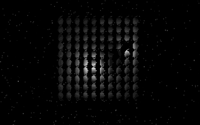
 First successful render! The math behind this isn’t that complicated, but I’d finally worked out enough of it to have something that could be called a “rendering engine”. Also, I’d gone through multiple languages and engines before I’d settled on doing it myself, so that took a while. Timestamp dates this to june ‘20 - I hadn’t noticed the irony of the first version successfully running on the first pride of the plague.
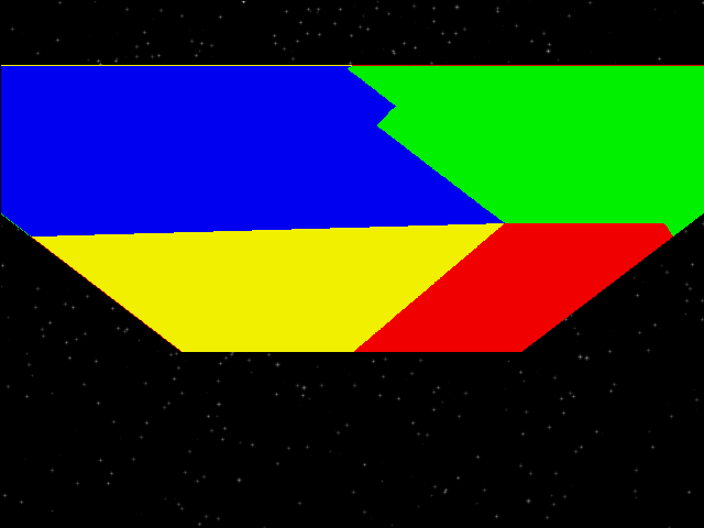
 First render with faces! This is from mid-‘20. You can still see gaps between the faces, that was an index error. I color-coded all the trisses so I could tell how they get rendered - lighting wasn’t a thing back then.
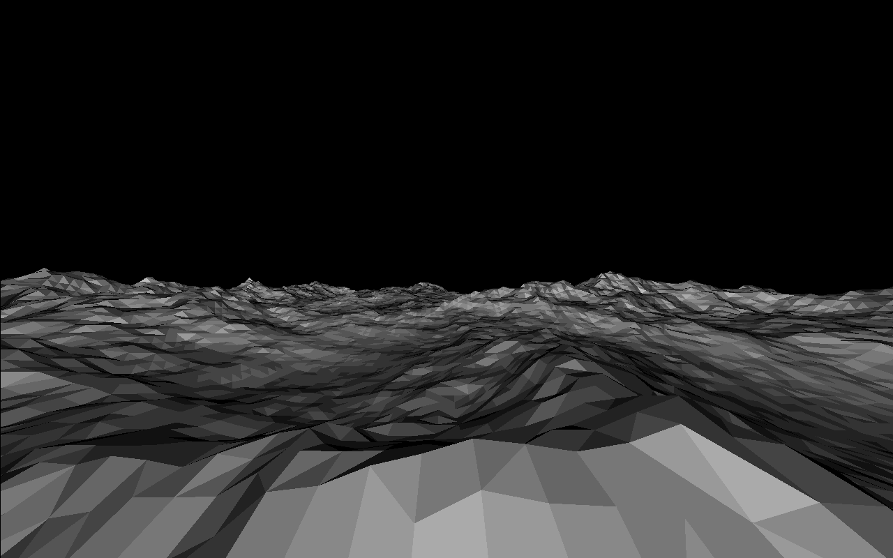 Now that I could render arbitrary models, I imported some perlin terrain from Blender to get some aesthetic shots.
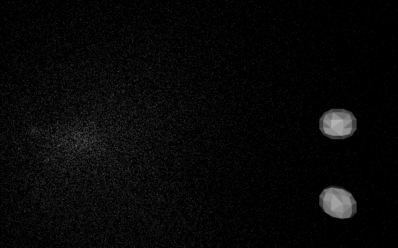 Rendering worked, basic lighting worked - time to set up the background! I downloaded and played around with the HYG database to figure out how the sky would look from TRAPPIST-1.
Now that we have the basics, I set off to coding orbital physics. A naive n-body solver is rather easy to make and fun to play with, but I’ll have to optimize it quite a bit if it’s to simulate an entire asteroid belt or the likes.
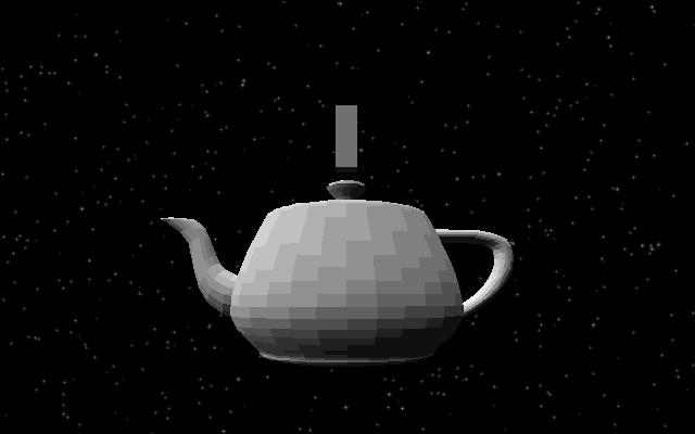 I lied - lighting didn’t work as it should! Took me a while to figure out I didn’t normalize face normals properly. Now it looks right.
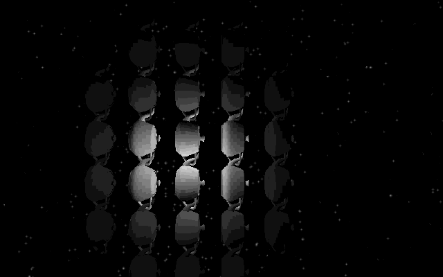
 Moar on lights - so far I just shaded triangles according to orientation to camera, so I sat down to implement a proper lighting system. It was inspired by LoZ:BotW, with a direct light and a sum of ambient lights, also cel shading (kind of enforced by the color space - there are only 16 light levels). What can I say, I’m a sucker for aesthetics. Now, if I can only get it to work reliably …
 Texture mapping! It is still affine - I implemented a fix for that, and then decided I liked the janky retro aesthetic more. It shouldn’t make a noticeable difference on any relevant level. P.S. I did end up fixing that later after implementing the depth buffer and realising it also solves this.